Successful market data projects require an understanding of how market data will be transformed. This week’s note provides an overview of the different approaches used to transform direct market quotes.
The valuation of an OTC derivative trade requires market prices to be fed into a model. The $valuation, i.e., present value (PV) output by the model is calculated by multiplying the trade’s expected cash flows (CFs) by the discount factors (DFs) applicable on the CF dates. To estimate the size of the CFs, forward rates for the underlying are used. If the derivative has optionality or is path-dependent, volatilities are required to derive the probabilities that the simulated CFs will be big enough to finish in-the-money.
Forward rates, discount factors and volatilities are the risk factors (RFs) of the model. Because markets are not infinitely liquid, observable quotes will not be available for many forward dates and strikes. Continuous curves and volatility surfaces solve this problem by fitting to the observable data.
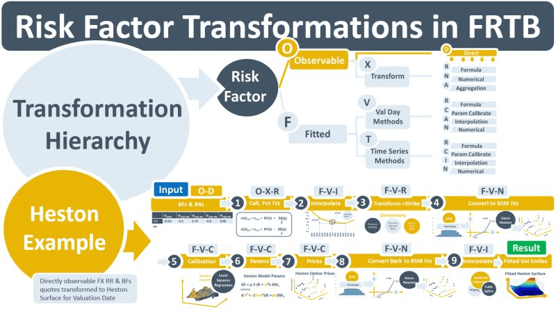
This means that there are two high-level categories of RFs in an FRTB ecosystem: observable and fitted. Within the observable category, there are two sub-categories: directly observable and transformed-observable. Within the fitted category, there are separate sub-categories: same-day-fitted and time-series-fitted. Within each of these categories, various types of RF transformation are possible: e.g., simple formulas applied to observable quotes, aggregation of quotes, numerical methods, interpolation, and model parameter calibration. The transformation categories have a hierarchical relationship as illustrated in the top of the diagram below.
The RF transformation process begins with directly observable quotes and involves multiple steps. Models can have three or more RFs, each one possibly containing a term structure and/or strike dimension. Different types of instruments can exist within the same term structure, each with its own quoting convention requiring a specific transformation.
When valuing e.g., an FX option, three RFs are required: the underlying spot rate, the volatility of the spot rate, and a yield curve containing the IR forward rates. If the model takes account of the changing, clustering nature of volatility then extra transformation steps are required to calibrate parameters that simulate the stochastic behaviour of volatility.
In the Heston model example below, directly observable FX risk-reversal and butterfly-structured option quotes obtained from brokers are input to the FX volatility transformation process. Nine transformation steps are required to convert them into a continuous Heston volatility surface – which becomes a fitted RF of the model. Each step in the example is coded so that it can be referenced to the transformation hierarchy.

