Bond pricing is central to market data projects. When bond prices are not liquid, modeling and proxy approaches are required. This week’s note discusses a framework for bond valuation.
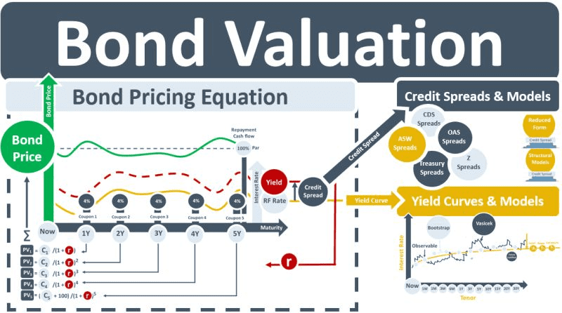
The issuer of a bond obtains a loan from the purchaser of the bond. The issuer agrees to pay regular coupons to the purchaser and repay the loan when the bond expires. The bond pricing equation (BPE) is used for two purposes. The first is to determine the coupon rate that will be attached to the bond at issuance. The coupon rate is the rate that results in a bond price of 100 for the prevailing bond yield. This coupon rate generates the fixed cash flows C1-C5 in the LH diagram above.
If the bond is traded in a liquid market, then post-issuance, there is no further need for the BPE because prices are freely available. If the bond is not liquid, however, the BPE is required to serve its second purpose, the calculation of the bond price using input yields. The valuation of the bond is calculated as the PV of its future CFs. The BPE generates PV1 by discounting the coupon C1 using the 1Y yield. PVs 2-5 are generated in the same way. PV5 includes the repayment of par. The sum of PVs 1-5 = the price of the bond, the green circle in the diagram.
The DFs used in the BPE are derived from the bond’s yield. But how are the yields obtained? Two approaches are possible: 1) a term structure of yields for the bond, and 2) a single yield for the bond.
For approach 1, the first step is to build an RF yc. Methods such as bootstrapping, Nelson-Siegel or Vasicek can generate a continuous curve of RF rates. Next, a credit spread (CS) reflecting the credit risk of the bond is added to each RF rate to determine the yields to use for discounting. The CS can be extracted from the prices of credit derivatives used to hedge the credit risk of bonds with similar credit characteristics to the bond being priced. CS types include asset swap spreads, CDS spreads, treasury spreads, z-spreads, and OAS spreads. A term structure of CSs is also possible. When CSs cannot be obtained from market instruments, models such as structural models or reduced-form models, allow credit spreads to be simulated.
Under approach 2, a single yield, referred to as the bond’s YTM or internal rate of return is used to discount all CFs in the BPE. Bonds with similar credit risk characteristics as the illiquid bond can be used to obtain the proxy YTM that is input to the BPE.
Over the life of the bond, the BPE will ensure that the bond’s price, the green wavy line in the diagram, will rise and fall in an opposing direction to its yield. As the bond matures, and time-to-maturity reduces, the impact of the changing YTM on the bond’s price gets smaller. Immediately before the bond matures, the time-to-maturity variable will be so small that changes in the bond’s yield have a negligible impact on its price. Assuming that there has been no credit event impacting the repayment of the par value of the bond, the bond’s price will move back to the 100 value at which it was issued.

