Time series of market data are used to generate shocks in market risk systems. The impact of changes in rates can have a non-linear relationship with generated OTC prices. This week’s email discusses convexity, a common non-linear impact of prices on output OTC prices referred to as convexity.
Models in finance require inputs, usually prices or parameters, to generate outputs which are often the prices of more complex financial instruments. The relationship between input values (horizontal axis) and output values (vertical axis), when plotted on a chart, will almost always exhibit curvature.
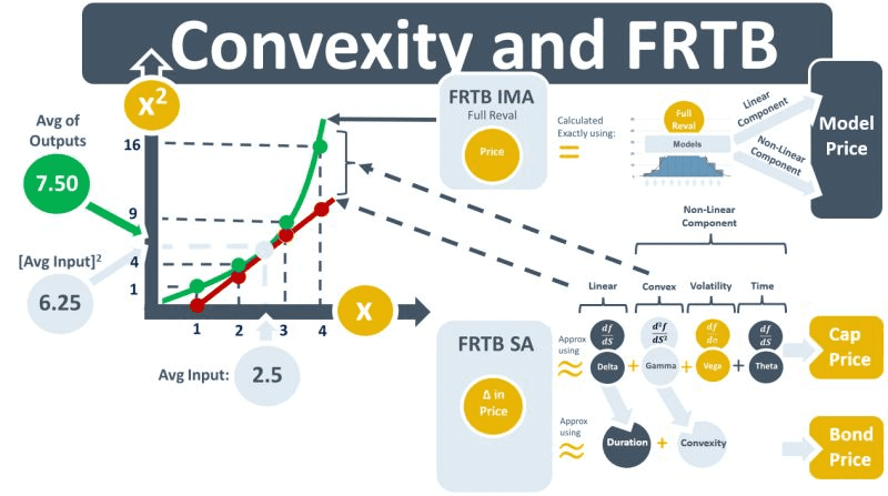
Convex functions, such as the x-squared fn in the diagram above, are a specific category of curves. They have the property that they always lie above tangent lines, e.g., the red line in the diagram, drawn to them. This accretive nature of convexity is formalized in a theory known as Jensen’s inequality. It states that the avg of the outputs generated by a convex fn is >= the fn’s output when the avg input value is used. The x-squared fn’s inputs in the diagram are 1, 2, 3, 4. The avg of those inputs is 2.5 and this number squared is 6.25. The fn’s outputs, however, are 1, 4, 9, and 16. And the avg of these outputs is 7.5. The outputs of the convex fn x-squared, therefore, have a greater avg value than transformed avg x-axis input value.
Two of the most common functions in QF, the call option fn and the bond yield-price fn, are also convex. Unlike x-squared, the QF functions contain random terms. The option fn transforms a random underlying price into a random price of an option written on it. The yield-price function transforms a random bond yield into a random bond price. In both cases, their randomness is the characteristic that enables the convexity to add value to the output prices. The pay-off function of a call option is convex because the holder benefits from price increases without facing similar losses when prices fall. Equivalently, bond prices are convex wrt changes in interest rates or yields because bond prices increase more when rates fall and they fall when rates rise. Yield-price convexity, therefore, offers some protection to bondholders in volatile interest rate environments. The more convexity in the relationship the more bond holders are protected.
The tangent line to the convex curve captures the change in the price of the output instruments for a small change in interest rates. This rate of change is known as IR delta for an option or duration for a bond. The convexity is referred to as gamma for the option and just convexity for the bond. The option has an additional exposure, vega, to the volatility of rates.
Under FRTB-SA, market risk capital is calculated by shocking rates by specified amounts and applying them to these risk sensitivities. Convexity is due to the asymmetry of the valuation impact of the difference between an upward and a downward shock of a rate. In FRTB IMA banks calculate their own rate shocks by simulating expected rate movements. Using the full reval approach, allowed under IMA, changes to all the instrument’s risk factors are done in a single run. The delta, duration, convexity, gamma, vega and theta as well as the cross effects on each other are calculated in parallel.

