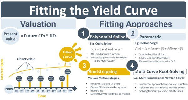
Quantitative transformations of different sorts are often in-scope for market data centralization projects. One generic type of transform is fitting yield curves. Data validated in the market data system are used as inputs for the fitting process. This week’s note discusses the different types of fitting approaches.
The present value, i.e., the valuation, of a derivative is calculated by multiplying its expected cash flows by the discount factors (DFs) applicable on those cash flow dates. While discount factors can be derived from observable market rates, they typically will not be available exactly on the dates of the cash flows. A continuous discount curve solves this problem. Discount factors, spot rates and forward rates can be derived from each other enabling a theoretical formula for the whole yield curve.
So, how is this continuous discount function calculated? One way to obtain continuous rates is to draw straight lines on a chart between the observable rates. This is referred to as linear interpolation. However, such a curve will not be smooth and when spot, forward and DF curves are derived from linearly interpolated rates they will lead to inconsistent valuations. Other interpolation or curve-fitting methods are therefore required. Four of the most common approaches are splines, parametric approaches, bootstrapping and multi-curve root-solving.
Spline methods assume that a curve can be modeled with a polynomial equation, e.g., if a cube (power of 3) term is the highest power in the equation then it is a cubic spline. Statistical regression techniques are used to estimate the coefficients of the polynomial. Curves are typically broken into segments joined at knots so that piecewise approaches to the spline-fitting can be taken. Parametric methods such as Nelson-Siegel, on the other hand, specify parameters that model aspects of the curve shape such as level, slope and curvature. Again, the parameters can be estimated using regression-type techniques. Bootstrapping methods are classical techniques that back DFs out of quotes for individual market instruments. The process is iterative, starting with instruments at the short-end and building up using longer-dated instruments. At each stage, a re-calibration is done to ensure that the set of derived DFs is consistent with the observable prices for the whole curve.
With the emergence post-crisis of the multi-curve framework and collateral-aware discounting, multiple input curves are now required to generate DF curves. The collateral allowable on the derivative’s CSA determines the type of discount curve and the problem of calculating the curves becomes a multi-dimensional one that requires DFs for all instruments across all curves to be calculated simultaneously while remaining consistent with market quotes. The problem can be characterized as a root-solving problem. One of the techniques used to solve it is a multi-dimensional Newton solver.

