The time-series of stock prices and the market-implied volatilities of stock prices are examples of market data that needs to be loaded and validated in a market data system. This week’s note discusses how the Heston stochastic volatility model interprets and uses the relationship between volatility as it is extracted from time-series data and volatility as it is observed in the market prices of options.
A deterministic process contains a quantity that changes over time exactly as specified by a formula. The formula S=t specifies that a stock price S will increase in a straight line with time. So, e.g., in 5 years the stock price will be five times higher. Lines with curvature mean that S changes in a non-linear, yet still pre-determined, way with time. If t is squared or raised to some power, the line for S will be curved and calculus needs to be used to determine how fast S is rising or falling or how quickly the curve is changing at any point in time.
Processes driven by human behaviour are never represented by straight lines and while curves can be good approximations, sometimes a random element needs to be added to the curve to accurately model behaviour. When that happens, the processes are no longer deterministic. Calculus needs to be replaced by stochastic calculus when estimating how fast S is rising or falling or how quickly curves are changing.
The most famous stochastic process in finance is geometric Brownian motion (GBM), developed in the 1950s. It adds a random term to a continuously compounding growth term. The random term contains a generated random-number multipled by a pre-set estimate of the stock’s volatility. The Black-Scholes option pricing model of the 1970s was based on GBM.
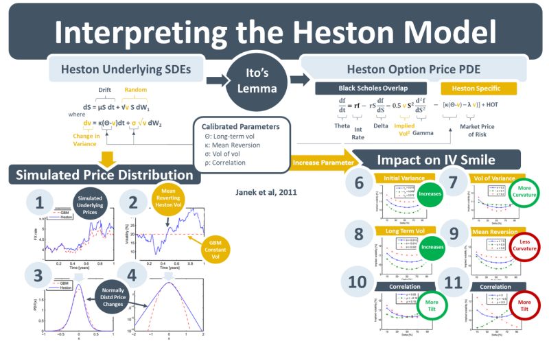
Researchers subsequently realised that pre-set, constant volatility was not a realistic assumption. Volatility clustered and varied over time. In 1993 Stephen Heston developed a model that accounted for the varying nature of volatility. While stock prices simulated by the Heston model do not look markedly different to those of GBM, they do exhibit more varying volatility – see 1 in the diagram below. Crucially though, in diagram 2, the GBM volatility parameter is flat whereas Heston volatility is random. Diagrams 3 and 4 show that under both GBM and Heston the changes in prices are normally distributed – a central assumption in quantitative finance.
Empirical analysis shows that volatility exhibits a long-term mean, reverts to that mean periodically, and has a negative correlation with stock prices because it increases when stock prices fall, and markets become scared. Heston-simulated stock prices and volatility can be controlled by the model’s parameters so that they align with movements in the historical time-series. Yet the parameters cannot simply be adjusted to reflect the historical data. Under no-arbitrage principles the option prices generated by the Heston model also need to be consistent with current market prices. Diagrams 6-11 below illustrate the impact that parameter adjustments have on the model-generated implied vols. Under no-arbitrage these need to match market-observed implied vols.