The Black Scholes model is used to generate implied volatilities – one of the main categories of market data. One of the key assumptions underlying the model is the lognormality of stock prices. This week’s note discusses the relationship between the lognormal assumption and the Black Scholes model.
Many data sets when arranged from the fewest occurrences to the largest and plotted on a histogram display roughly as a bell shape known as the normal distribution (ND). In finance, daily stock price changes are typically ND. Lognormally distributed (LND) data such as stock prices (i.e., not stock price changes), on the other hand, cannot go below zero and are therefore not symmetric and bell-shaped. ND and LND observed data can be simulated mathematically using probability density functions (PDFs) which generate smooth curves that fit the observed distributions. The mean, µ, and standard deviation, σ, are parameters of the PDFs.
Models in quantitative finance use PDFs when estimating probabilities that cash flows will occur. Models that use the ND PDF are easier to find solutions for than models that use LND PDF. The model used for stock price changes is geometric Brownian motion (GBM). It assumes that stock price changes, dS, are generated using a deterministic term, µSdt, +/- increments from a random term, σSdW. Because the deterministic term continuously multiplies µ, the growth rate, by S, the stock price, the resulting stock price will compound and increase over time. The increasing stock price will result in larger and larger stock price changes that will lead to those changes exhibiting an LND rather than an ND.
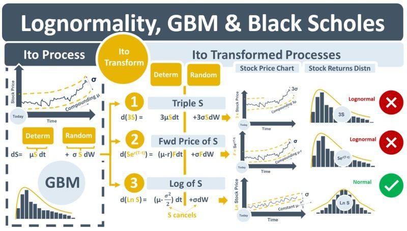
GBM is an example of a stochastic differential equation (SDE) that is an Ito process. It models the change over time in S, dS. Ito’s lemma states that any function of S will result in another Ito process when after an Ito transformation. The diagram below shows GBM on the LHS. The RHS contains three examples of GBM being Ito-transformed. dS is transformed into d(3S), d(forward price of S) and d(Ln S). The problem with the first two examples is that post-transformation, their terms still contain S – the transformed processes will still be geometric and lognormal. Example 3, however, is different. It is Ln S, the natural log of S. When GBM is transformed into d(Ln S), it results in an Ito process that no longer contains S in its terms. This removes the compounding from the stock price changes and the “G” from GBM. The resulting SDE generates price changes that are ND which makes it easier to use in option pricing models like the Black-Scholes-Merton (BSM) model.
The BSM equation is famously derived using no-arbitrage arguments that remove the troublesome growth rate, μ, parameter from GBM. Despite the removal of μ from GBM getting all the credit, the removal of S from the terms of the Ito-transformed GBM, however, is equally important. Without it, solutions to the BSM PDE, i.e., the BSM formulas, would not be possible.