We are working on enhancing time series validation for curves at the moment. One of the use cases for the time series of curves is PCA. Principal components can also be used in the validation of the time-series. This led me to write this week’s email on the background to PCA and the term structure.
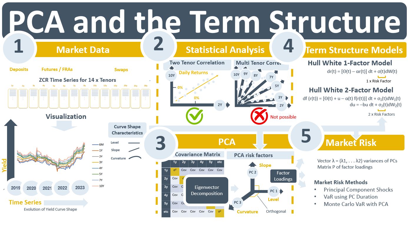
A yield curve containing, say 14 tenors, typically makes a parallel movement, or close to it, between one day and the next. This means that when the time series of the 14 tenors are examined statistically the daily returns on, say, the 2Y rate will be highly correlated with those of, say, the 10Y rate. The “two tenor correlation” chart in the diagram below is an illustration of this. In fact, all of the possible pair-wise tenor combinations will have high correlation values. If we moved to three dimensions correlations are not possible but a 3-D chart can be plotted showing a regression line through the “swarm” of return observations from the combined say 2Y, 5Y, and 10Y time series. Beyond three dimensions visualizing relationships between time series is not possible. So, for analysing the relationships in the full data set we have to resort to a 2-D plot of all of the data.
Statistically, all of those pair-wise relationships can be captured in a single construct such as the covariance or correlation matrix. However, the covariance matrix table contains a lot of data. The human eye cannot read it and infer what the yc’s real risk factors are. A review of the 2-D time series chart for all tenors would indicate that the bank has exposures to 1) a change in the level of the curve, 2) a change in its slope, or 3) a change in how much it bends. Can such a heuristic approach to risk management be correct? It turns out that it can and that it can be proven using a statistical technique called principal component analysis (PCA).
The purpose of PCA is to estimate the covariance matrix. It does so by drawing lines for each tenor in 14-D space that are centred by unit variance and orthogonal to each other. The explanatory power of the covariance matrix is allocated to the 14 orthogonal lines using eigenvectors. The result is an estimation of the risk factors of the yc. These risk factors are referred to as principal components (PCs). For highly correlated data like that in yc series, the explanatory power will be fully allocated after three iterations with PC1 being the risk factor for a change in the level of interest rates, PC2 being the slope factor and PC3 the curvature factor.
PCA emerged as a technique for yield curve analysis in the 1990s and 2000s. It proved that, in the fixed income and rates world, more than just a single “short rate” random variable was required to estimate the term structure. Around the same time, term structure models such as Hull White began to move from 1-factor models based on that single short rate to assuming there were two and maybe even three risk factors associated with a yc. In market risk, variations on techniques such as parametric and Monte Carlo VaR were developed to take advantage of PCA. A yc could be shocked by its PCs when estimating the valuation impact of its movements under different scenarios.