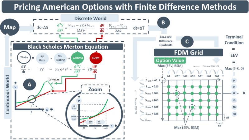
The BSM equation describes how an option value, V, changes over time (dV/dt). It is a PDE that describes the inter-relationships of multiple variables. The most important relationship is the one btw the underlying price (say a stock price, S) and the value V of the option written on it. The green line in diagram A illustrates the relationship for a call option. As S rises so does V. It is a smooth, but non-linear relationship. At the strike price K, V begins to rise at a faster rate, rising to the point that it becomes a 45-degree angle on the S-V axis. At this point S is deep in-the-money. The green line has a slope of 1 and V and S are now behaving like they belong to the same traded instrument.
The red line is a tangent to the green line. It can be used to approximate how much V changes for a small change in S, dS. The red tangent line is touching the green curve at the strike price K implying the stock price S in the example is at-the-money. This slope of the red line is the delta of the option. The difference btw the green and red line is the curvature of the option. Curvature determines a) how quickly delta changes and b) the size of the curvature error when delta is used to approximate changes in the option value for a given change in S. The curvature of an option is also known as its gamma.
American options can be exercised on any date btw now and their maturity. A call option holder will exercise if they think that the early exercise value, Max(S-K, 0), is greater than the BSM-calculated value. When valuing an American option, a method is therefore needed which compares the EEV to the BSM value on each day prior to the maturity date. An FDM grid achieves this. It maps the multi-variate relationships in the BSM continuous world to an equivalent set of relationships in the BSM discrete world. In this discrete world a plausible range for S is divided into fixed price intervals, ΔS. The time-to-maturity T is divided into daily time intervals, ΔT. The nodes of the FDM grid (C below) contain the BSM option prices for each combination of ΔS and ΔT.
FDMs take advantage of the fact that the terminal value V for the call option is known given the forward price of S. That is, V = max (S-K, 0). The FDM then works backwards from the terminal date to determine the BSM option values V(ΔS, ΔT) at each node on the grid. It does this using the discrete world version of the BSM PDE. In this world of time-steps and fixed stock price increments, delta and gamma are calculated using BSM difference quotients (see B) and plugged into the discrete BSM PDE.
As the discrete BSM PDE works backwards from the terminal value, the option value at each node is calculated as the max of the EEV & the BSM value. The difference eqn keeps working backwards an upwards until the node at the top LHS of the grid is reached. The value of this node is the price of the American call option.