At GoldenSource we are working on some projects that involve the sourcing and validating of cap-floor data. The data primarily comes from brokers who make two-way markets in caps and floor trades. They sell the resulting market data to banks and other customers who use the data to price their derivative portfolios. This week’s note talks about how cap-floor data is used when pricing interest rate derivatives.
A cap is a type of interest rate option. It gives the holder the right to receive payments if the interest rate (IR) rises above the strike price. A floor pays if the IR falls below the strike. Caps and floors are liquid OTC IR options. Their vanilla nature means they can be valued using standard Black-Scholes-Merton (BSM)-type models.
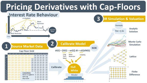
However, the BSM model has two limiting assumptions. The first is it assumes that the volatility of an IR is constant over time. This is incorrect. Empirical evidence tells us that IR volatility changes over time. It is stochastic and typically arrives in clusters. The second is that the IR is flat over time. Again, this is incorrect. An IR has a term structure that contains different, though highly correlated, IRs depending on the length of time that money is lent. Cap and floor prices modelled using BSM are displayed on a grid by the brokers and banks advertising their quotes. Implied volatility (IVs) can be derived from either cap or floor prices. The convention is for the grid to contain floor prices (or IVs) for lower strikes and cap prices (or IVs) for higher strikes. When plotted on a 3-D chart using the tenor and strike as the axes, the grid becomes a surface. The brokers, e.g., ICAP or Tullets, who advertise the prices, specify the conventions they use when calculating the cap and floor prices.
The IV content of the cap-floor grid leads to the grid having a second purpose. It is used to calibrate the parameters of models that have evolved to attempt to address these two limiting assumptions (constant volatility, constant IR) of BSM. The grid in the diagram below has two dimensions, a strike dimension and a term structure dimension which contain information on changes in volatility due to a) the term structure, and b) the random nature of IR volatility. The Hull-White (HW) model is a commonly used model for the behaviour of IR, i.e. dr(t), as it changes over time. The stochastic differential equation (SDE) that underlies it contains three parameters, long-term mean, mean-reversion, and volatility. Calibrating these parameters requires tuning them until the model re-prices exactly all of the options on the cap-floor grid. By doing so, the parameters are infused with the information that the grid contains on both term structure and the randomness of the IR’s volatility. The tendency of the IR to mean-revert to its term structure trajectory is also captured. With its parameters thus infused, the SDE is empowered to act as the basis for the modelling and simulation of the IR over time. Analytical solutions to the PDE, Monte Carlo simulation, lattice methods, and finite difference methods are the four main approaches that use the SDE.