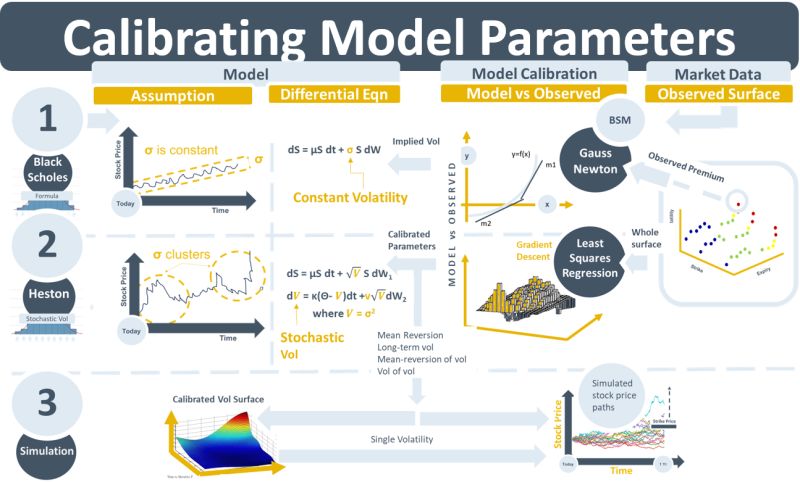
One of the main functions of market data that exists on curves or surfaces is for use in calibrating model parameters. This week’s note discusses the background to and process of calibrating model parameters that are used in derivatives pricing.
If a bond market was so deep and liquid that it had prices available continuously for all maturities, then there would be no need to fit a yield curve to it. If a related options market was equally deep and liquid and contained option prices for a continuous set of strikes and expiries far out into the future, there would be no need to fit an implied volatility surface to it. But markets are not that liquid. Curve and surface fitting is therefore a core activity in quantitative finance. When curves are fit, they are, by definition, continuous, and prices can be derived from them for all maturities and strikes.
Curve fitting is done with an equation. The equation y=x predicts that y, the dependent variable, will grow at the same rate as x, the explanatory variable. It plots as a 45-degree line on the x-y chart. y=2x predicts that y will always be twice as large as x. It plots as a 60-degree line. The number “2” is the coefficient in this equation. Sometimes y is dependent on two variables, x and z. Sometimes more. Sometimes the explanatory variables are squared or have higher powers. When they do, the line plotted will be non-linear.
In quantitative finance these equations are models. The y-value that is being predicted and whose curve is being fit, might e.g., be an interest rate. The coefficients of the equations, instead of being explicit numbers, are replaced with either variables or parameters. When the model is run the variables are taken from liquid, daily changing, observable data such as a stock price. Parameters, on the other hand, are not taken directly from the market. Instead, they need to be adjusted so that the curves best fit the observed data. This optimization process is called model calibration. Various optimization processes exist, such as Gauss-Newton (GN), Gradient-Descent (GD), or Levenberg-Marquardt (LM).
The most important model parameter in the world of derivatives pricing is implied volatility. It impacts the value of all traded instruments that have embedded or explicit optionality. The GN optimization method is used to solve for the single implied volatility number that best fits an observed option price when the Black-Scholes-Merton model is used to calculate the option price. When the fitting of the entire set of option prices or implied volatilities for a surface is required, then the problem is typically formulated as a non-linear least squares optimization problem. The objective though is still the same: fit the curves and contours of the surface as best as possible to the observed prices. The GD and LM methods are used to solve for model parameters that minimize the sum of the squared differences between the fitted curves and the observed data.