Building market data systems that produce market rates for use in bank’s derivative pricing libraries requires an understanding of some of the assumptions behind the market rates that are produced on trading venues. A key assumption behind all market rates and the model parameters that are calibrated to those market rates, is that they are risk neutral. The concept of risk-neutral valuations is summarised in this week’s note.
A 10% change in price, e.g., a 10% daily return, for a blue-chip stock is a more unusual event than a 10% change on a high-risk small-cap stock. Investment managers use the Sharpe ratio, λ, to compare these two price changes. The ratio, which divides the return minus the risk-free rate (µ-r) by the standard deviation of the stock, σ, allows the price-changes of the two stocks to be compared from a risk-adjusted perspective. Another term for the Sharpe ratio is the market price of risk (MPR).
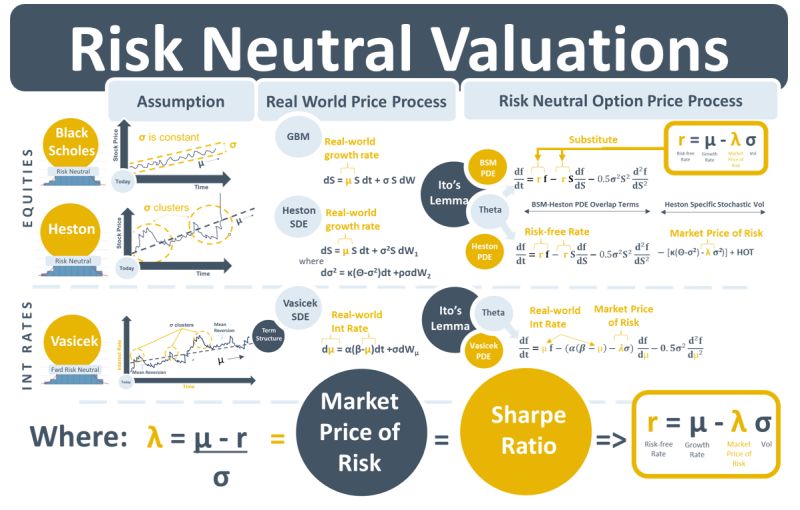
The core approach in option pricing mathematics is the use of Ito’s lemma to convert a process for stock price movements, (visualise a stock price chart), into a process for option price movements, (visualise a chart showing the price of an option on that stock). For example, the Black-Scholes-Merton (BSM) model converts the geometric Brownian motion (GBM) stock price process into an option price process that is described by the BSM partial differential equation (PDE). The Heston model converts a random-volatility stock price process into a Heston option price PDE, and the Vasicek model converts a mean-reverting random interest rate process into a Vasicek PDE.
The standard deviation, σ, aka implied volatility, underlies both the MPR equation and option pricing models. Re-arranging the MPR equation, we get r = µ – λσ, so that when there is no market price risk in the stock, i.e., λσ=0, we are left with r=µ, i.e., the return of the stock = the risk-free rate. This r=µ assumption is central to the BSM model. It can be made because of no-arbitrage arguments that underlie the model. If the stock price movement is assumed to be perfectly hedged by the option price movement, it means there is no market risk in the portfolio, which can be assumed then to grow at the risk-free rate r. This makes the model much simpler to use because stock price growth, μ, does not have to be estimated. The concept of converting real-world growth rates into risk-free rates using no-arbitrage arguments is referred to as risk-neutral valuations.
The MPR equation also comes into derivative pricing models that evolved from BSM. In Heston, like BSM, the MPR is assumed to be zero for its PDE terms that overlap with BSM. The non-overlapping terms that control how Heston volatility changes over time, however, do need to be adjusted for the MPR. The option price PDEs in term structure models such as the Vasicek model also include adjustments for the MPR.
The MPR, like all model parameters, needs to be estimated before running any model that include it. Where possible this is done by calibrating to observable market data.