Users and testers on market data projects often come from the areas of market risk, IPV, and P&L. This week’s note talks about how a mathematical concept known as a Taylor series approximation is the underlying technique that is used to estimate the P&L impact of daily changes or differences in market data.
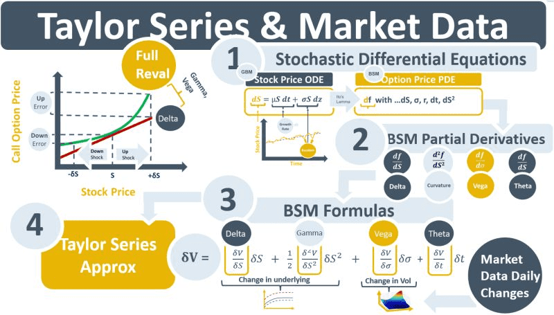
One of the objectives of market risk and P&L analysis is to be able to apply changes in market prices to the risk factors of a derivative pricing model that are exposed to those changes to determine the P&L impact of the changes. This is challenging because the pricing model takes all of the risk factor inputs, merges them and models the interactions between them to estimate and discount future cash flows to produce a single “full reval” derivative price in a way that is not transparent to the user. Taylor polynomial approximations help with this challenge. They allow users to apply market data changes directly to a model’s risk factors.
In mathematics, a function can often be represented by an infinite polynomial, aka a power series. E.g., the non-linear function 1/(1-x) is represented by the series 1 + x + x^2 + x^3 + …. + x^n. Taylor series is a technique for generating infinite polynomials using derivatives of the function. Once generated, the first few terms of the Taylor polynomial can be used to approximate the behaviour of the fn.
An option’s price, the green line in the LH diagram below, is a non-linear fn of its underlying stock price. The stock’s delta, the red line, approximates the change in the option price as the stock price changes but it does not capture the curvature. The main components of the curvature are gamma and vega. Gamma captures the impact of a change in delta. Vega captures the impact of a change in observed implied volatility.
Delta, gamma and vega are partial derivatives of the Black-Scholes-Merton (BSM) stochastic differential equation (SDE). One of the benefits of the BSM framework is that it comes with a formula that calculates the price of an option. The formula calculates the single full reval price of the option after modelling the impact and relationships between its risk factors. Embedded in the full reval price, therefore, is the impact of all the partial derivatives of the BSM SDE. BSM also comes with relatively simple formulas for calculating the option’s delta, vega and gamma, which are the option’s Greeks or risk sensitivities.
Using a Taylor expansion, the full reval price calculated by the BSM formula can be re-constructed from its risk factors using risk sensitivities. This is achieved by plugging the calculated delta, gamma and vega numbers into the abbreviated Taylor polynomial. The result should be an option price vs stock price curve that approximates the full reval curvature of the green line in the diagram. Daily changes in market data can then be applied to the sensitivities using the terms of the Taylor polynomial.
Risk-sensitivity-based approaches for controls such as IPV, VaR, bid-ask reserves, P&L attribution, and prudential valuations require the use of Taylor series approximations. They are typically less computationally expensive than full reval approaches.